(tensorflow v2.4.0)
Fully Convolutional Network(FCN)를 사용해서 Image Segmentation을 수행하는 모델을 구현해보도록 하겠습니다.
먼저 FCN에 대해서 아주 간단하게 살펴보겠습니다. FCN의 자세한 내용은 논문을 참조하시기 바랍니다.(paper)
Fully Convolutional Networks(FCN)

논문의 제목에서 나타나듯이, FCN은 Image Segmentation을 위해 만들어진 네트워크입니다.
네트워크는 위 이미지처럼 Image를 입력으로 받고, 일반적인 Conv Block(Conv - Pooling) 구조를 여러층으로 쌓아서 Feature extractor를 구성하고, 추출된 feature들을 Fully-connected layer가 아닌 Conv layer를 사용해서 이미지의 segmentation heatmap을 예측합니다.(feature extractor를 Encoder, Heatmap 추출을 Decoder라고 부릅니다.)
이때, 결과로 나오는 heatmap은 각 픽셀(pixel)에서 각 클래스의 확률 정보를 담고있습니다.
여기서, 일반적인 방법의 CNN 구조로는 결과의 해상도가 너무 낮기 때문에 정확한 해상도를 가지는 Segmentation이 불가능합니다. 따라서, Deconvolution을 통한 Upsampling을 통해서 heatmap을 원본 이미지의 크기와 동일하게 만들어주는 과정이 Decoder에 포함됩니다.
Skip Connection

그리고 Decoder에서의 Upsampling 과정에서 Skip Connection 기법을 사용합니다. Pooling이 진행될수록 낮아지는 해상도를 높이기 위해서 이전 Pooling layer를 활용하는 아이디어입니다.
여기서 FCN-32s, FCN-16s, FCN-8s로 세 가지의 결과를 출력할 수 있는데, 숫자는 사용한 Stride를 의미합니다.
즉, 마지막 pool5 layer만을 사용하여 Upsampling(Stride = 32) 진행하면 FCN-32s 결과가 출력됩니다.
FCN-16s의 경우에는 pool5를 2x upsampling을 진행하고, 이전 pool layer인 pool4와 더한 뒤에 16x Upsampling을 진행하게 됩니다.
FCN-8s는 앞서 2x upsampling한 pool5와 pool4를 더한 결과를 다시 2x sampling을 진행하고, 이전 pool3 layer와 더한 후에 8x upsampling을 진행한 결과입니다.

FCN-8s로 갈수록 정확도가 더 올라가는 것을 볼 수 있습니다.
이제 FCN 네트워크를 직접 구현해볼텐데, pre-trained VGG-16 네트워크를 사용해서 학습을 진행할 예정입니다.
사용되는 dataset은 Link에서 제공하는 data를 사용하였습니다.
(jupyter notebook에서는 coursera에서 제공되는 경로로 다운로드합니다.)
Import
필요한 package들을 import하고 시작해보도록 하겠습니다.
import os
import zipfile
import PIL.Image, PIL.ImageFont, PIL.ImageDraw
import numpy as np

import tensorflow as tf
import tensorflow_datasets as tfds
import matplotlib.pyplot as plt
import seaborn as sns

print('Tensorflow version ' + tf.__version__)
Download the Dataset
# download the dataset (zipped file)
!wget --no-check-certificate \
    https://storage.googleapis.com/laurencemoroney-blog.appspot.com/fcnn-dataset.zip \
    -O /content/fcnn-dataset.zip

# extract the downloaded dataset to a local directory: /tmp/fcnn
local_zip = '/content/fcnn-dataset.zip'
zip_ref = zipfile.ZipFile(local_zip, 'r')
zip_ref.extractall('/content/fcnn')
zip_ref.close()
저는 Google Colab으로 진행했는데, Local에서 진행하신다면 위의 data link를 통해서 직접 다운받으셔서 진행할 수 있습니다.
Load and Prepare the Dataset
data에서 사용되는 class는 총 12개이며, annotation image(label map)의 픽셀값은 각 class에 해당되는 값으로 되어있습니다.
# pixel labels in the video frames
class_names = ['sky', 'building','column/pole', 'road', 'side walk', 'vegetation', 'traffic light', 'fence', 'vehicle', 'pedestrian', 'bicyclist', 'void']
Training/Validation Dataset을 만들기 전에 필요한 함수들을 정의하고, Dataset을 만들겠습니다.
train_image_path = '/content/fcnn/dataset1/images_prepped_train/'
train_label_path = '/content/fcnn/dataset1/annotations_prepped_train/'
test_image_path = '/content/fcnn/dataset1/images_prepped_test/'
test_label_path = '/content/fcnn/dataset1/annotations_prepped_test/'

BATCH_SIZE = 64
Dataset을 위한 함수들은 더보기를 클릭해주세요.
def map_filename_to_image_and_mask(t_filename, a_filename, height=224, width=224):
    '''
    Preprocesses the dataset by:
        * resizing the input image and label maps
        * normalizing the input image pixels
        * reshaping the label maps from (height, width, 1) to (height, width, 12)

    Args:
        t_filename(string) -- path to the raw input image
        a_filename(string) -- path to the raw annotation (label map) file
        height(int) -- height in pixels to resize to
        width(int) -- width in pixels to resize to

    Returns:
        image(tensor) -- preprossed image
        annotation(tensor) -- preprocessed annotation
    '''

    # Convert image and mask files to tensors
    img_raw = tf.io.read_file(t_filename)
    anno_raw = tf.io.read_file(a_filename)
    image = tf.image.decode_jpeg(img_raw)
    annotation = tf.image.decode_jpeg(anno_raw)

    # Resize image and segmentation mask
    image = tf.image.resize(image, (height, width,))
    annotation = tf.image.resize(annotation, (height, width,))
    image = tf.reshape(image, (height, width, 3,))
    annotation = tf.cast(annotation, dtype=tf.int32)
    annotation = tf.reshape(annotation, (height, width, 1,))
    stack_list = []

    # Reshape segmentation masks
    for c in range(len(class_names)):
        mask = tf.equal(annotation[:,:,0], tf.constant(c))
        stack_list.append(tf.cast(mask, dtype=tf.int32))

    annotation = tf.stack(stack_list, axis=2)

    # Normalize pixels in the input image
    image = image / 127.5
    image -= 1

    return image, annotation

def get_dataset_slice_paths(image_dir, label_map_dir):
    '''
    generates the lists of image and label map paths

    Args:
        image_dir (string) -- path to the input images directory
        label_map_dir (string) -- path to the label map directory

    Returns:
        image_paths (list of strings) -- paths to each image file
        label_map_paths (list of strings) -- paths to each label map
    '''

    image_file_list = os.listdir(image_dir)
    label_map_file_list = os.listdir(label_map_dir)
    image_paths = [os.path.join(image_dir, fname) for fname in image_file_list]
    label_map_paths = [os.path.join(label_map_dir, fname) for fname in label_map_file_list]

    return image_paths, label_map_paths

def get_training_dataset(image_paths, label_map_paths):
    '''
    Prepares shuffled batches of the training set.

    Args:
        image_dir (string) -- path to the input images directory
        label_map_dir (string) -- path to the label map directory

    Returns:
        tf Dataset containing the preprocessed train set
    '''
    training_dataset = tf.data.Dataset.from_tensor_slices((image_paths, label_map_paths))
    training_dataset = training_dataset.map(map_filename_to_image_and_mask)
    training_dataset = training_dataset.shuffle(100, reshuffle_each_iteration=True)
    training_dataset = training_dataset.batch(BATCH_SIZE)
    training_dataset = training_dataset.repeat()
    training_dataset = training_dataset.prefetch(-1)

    return training_dataset

def get_validation_dataset(image_paths, label_map_paths):
    '''
    Prepares shuffled batches of the validation set.

    Args:
        image_dir (string) -- path to the input images directory
        label_map_dir (string) -- path to the label map directory

    Returns:
        tf Dataset containing the preprocessed train set
    '''
    validation_dataset = tf.data.Dataset.from_tensor_slices((image_paths, label_map_paths))
    validation_dataset = validation_dataset.map(map_filename_to_image_and_mask)
    validation_dataset = validation_dataset.batch(BATCH_SIZE)
    validation_dataset = validation_dataset.repeat()

    return validation_dataset
# get the paths to the images
training_image_paths, training_label_map_paths = get_dataset_slice_paths(train_image_path, train_label_path)
validation_image_paths, validation_label_map_paths = get_dataset_slice_paths(test_image_path, test_label_path)
# generate the train and valid sets
training_dataset = get_training_dataset(training_image_paths, training_label_map_paths)
validation_dataset = get_validation_dataset(validation_image_paths, validation_label_map_paths)
다음으로는 각 클래스의 segmentation 색상을 지정하도록 하겠습니다. seaborn의 color_pallette를 사용해서 RGB값을 불러옵니다.
# generate a list that contains one color for each class
colors = sns.color_palette(None, len(class_names))

# print class name - normalized RGB tuple pairs
# the tuple values will be multiplied by 255 in the helper functions later
# to convert to the (0,0,0) to (255,255,255) RGB values you might be familiar with
for class_name, color in zip(class_names, colors):
    print(f'{class_name} -- {color}')
아래 함수들은 시각화를 위한 함수입니다.(더보기 클릭)
# Visualization Utilities

def fuse_with_pil(images):
    '''
    Creates a blank image and pastes input images

    Args:
        images (list of numpy arrays) - numpy array representations of the images to paste

    Returns:
        PIL Image object containing the images
    '''

    widths = (image.shape[1] for image in images)
    heights = (image.shape[0] for image in images)
    total_width = sum(widths)
    max_height = max(heights)

    new_im = PIL.Image.new('RGB', (total_width, max_height))

    x_offset = 0
    for im in images:
        pil_image = PIL.Image.fromarray(np.uint8(im))
        new_im.paste(pil_image, (x_offset,0))
        x_offset += im.shape[1]

    return new_im


def give_color_to_annotation(annotation):
    '''
    Converts a 2-D annotation to a numpy array with shape (height, width, 3) where
    the third axis represents the color channel. The label values are multiplied by
    255 and placed in this axis to give color to the annotation

    Args:
        annotation (numpy array) - label map array

    Returns:
        the annotation array with an additional color channel/axis
    '''
    seg_img = np.zeros( (annotation.shape[0],annotation.shape[1], 3) ).astype('float')

    for c in range(12):
        segc = (annotation == c)
        seg_img[:,:,0] += segc*( colors[c][0] * 255.0)
        seg_img[:,:,1] += segc*( colors[c][1] * 255.0)
        seg_img[:,:,2] += segc*( colors[c][2] * 255.0)

    return seg_img


def show_predictions(image, labelmaps, titles, iou_list, dice_score_list):
    '''
    Displays the images with the ground truth and predicted label maps

    Args:
        image (numpy array) -- the input image
        labelmaps (list of arrays) -- contains the predicted and ground truth label maps
        titles (list of strings) -- display headings for the images to be displayed
        iou_list (list of floats) -- the IOU values for each class
        dice_score_list (list of floats) -- the Dice Score for each vlass
    '''

    true_img = give_color_to_annotation(labelmaps[1])
    pred_img = give_color_to_annotation(labelmaps[0])

    image = image + 1
    image = image * 127.5
    images = np.uint8([image, pred_img, true_img])

    metrics_by_id = [(idx, iou, dice_score) for idx, (iou, dice_score) in enumerate(zip(iou_list, dice_score_list)) if iou > 0.0]
    metrics_by_id.sort(key=lambda tup: tup[1], reverse=True)  # sorts in place

    display_string_list = ["{}: IOU: {} Dice Score: {}".format(class_names[idx], iou, dice_score) for idx, iou, dice_score in metrics_by_id]
    display_string = "\n\n".join(display_string_list)

    plt.figure(figsize=(15, 4))

    for idx, im in enumerate(images):
        plt.subplot(1, 3, idx+1)
        if idx == 1:
            plt.xlabel(display_string)
        plt.xticks([])
        plt.yticks([])
        plt.title(titles[idx], fontsize=12)
        plt.imshow(im)


def show_annotation_and_image(image, annotation):
    '''
    Displays the image and its annotation side by side

    Args:
        image (numpy array) -- the input image
        annotation (numpy array) -- the label map
    '''
    new_ann = np.argmax(annotation, axis=2)
    seg_img = give_color_to_annotation(new_ann)

    image = image + 1
    image = image * 127.5
    image = np.uint8(image)
    images = [image, seg_img]

    images = [image, seg_img]
    fused_img = fuse_with_pil(images)
    plt.imshow(fused_img)


def list_show_annotation(dataset):
    '''
    Displays images and its annotations side by side

    Args:
        dataset (tf Dataset) - batch of images and annotations
    '''

    ds = dataset.unbatch()
    ds = ds.shuffle(buffer_size=100)

    plt.figure(figsize=(25, 15))
    plt.title("Images And Annotations")
    plt.subplots_adjust(bottom=0.1, top=0.9, hspace=0.05)

    # we set the number of image-annotation pairs to 9
    # feel free to make this a function parameter if you want
    for idx, (image, annotation) in enumerate(ds.take(9)):
        plt.subplot(3, 3, idx + 1)
        plt.yticks([])
        plt.xticks([])
        show_annotation_and_image(image.numpy(), annotation.numpy())
Dataset의 이미지들은 다음과 같습니다.
list_show_annotation(training_dataset)
Define the Model
먼저 Encoder를 구성해보도록 하겠습니다. 사전 학습된 VGG-16 Network를 사용할 예정이므로, VGG-16의 구조를 먼저 구성합니다. Conv - Pooling layer의 block이 반복되므로, Block을 구성하는 함수를 구현하고 전체 Encoder를 구현하겠습니다.

def block(x, n_convs, filters, kernel_size, activation, pool_size, pool_stride, block_name):
    '''
    Defines a block in the VGG block

    Args:
        x(tensor) -- input image
        n_convs(int) -- number of convolution lyaers to append
        filters(int) -- number of filters for the convolution lyaers
        activation(string or object) -- activation to use in the convolution
        pool_size(int) -- size of the pooling layer
        pool_stride(int) -- stride of the pooling layer
        block_name(string) -- name of the block

    Returns:
        tensor containing the max-pooled output of the convolutions
    '''
    for i in range(n_convs):
        x = tf.keras.layers.Conv2D(filters=filters,
                                   kernel_size=kernel_size,
                                   activation=activation,
                                   padding='same',
                                   name=f'{block_name}_conv{i+1}')(x)

    x = tf.keras.layers.MaxPooling2D(pool_size=pool_size,
                                     strides=pool_stride,
                                     name=f'{block_name}_pool{i+1}')(x)

    return x
그리고 학습된 VGG-16의 weight를 다운받습니다.
# download the weights
!wget https://github.com/fchollet/deep-learning-models/releases/download/v0.1/vgg16_weights_tf_dim_ordering_tf_kernels_notop.h5

# assign to a variable
vgg_weights_path = "vgg16_weights_tf_dim_ordering_tf_kernels_notop.h5"
VGG-16 Network 구현
입력의 shape는 (224,224,3)이며, block 함수를 통해서 VGG-16 네트워크를 구현합니다.
def VGG_16(image_input):
    '''
    This function defines the VGG encoder.

    Args:
        image_input(tensor) -- batch of images

    Returns:
        tuple of tensors -- output of all encoder blocks plus the final convolution layer
    '''

    # create 5 blocks with increasing filters at each stage
    x = block(image_input, n_convs=2, filters=64, kernel_size=(3,3), activation='relu',
              pool_size=(2,2), pool_stride=(2,2),
              block_name='block1')
    p1 = x # (112, 112, 64)

    x = block(x, n_convs=2, filters=128, kernel_size=(3,3), activation='relu',
              pool_size=(2,2), pool_stride=(2,2),
              block_name='block2')
    p2 = x # (56, 56, 128)

    x = block(x, n_convs=3, filters=256, kernel_size=(3,3), activation='relu',
              pool_size=(2,2), pool_stride=(2,2),
              block_name='block3')
    p3 = x # (28, 28, 256)

    x = block(x, n_convs=3, filters=512, kernel_size=(3,3), activation='relu',
              pool_size=(2,2), pool_stride=(2,2),
              block_name='block4')
    p4 = x # (14, 14, 512)

    x = block(x, n_convs=3, filters=512, kernel_size=(3,3), activation='relu',
              pool_size=(2,2), pool_stride=(2,2),
              block_name='block5')
    p5 = x # (7, 7, 512)

    # create the vgg model
    vgg = tf.keras.Model(image_input, p5)

    # load the pretrained weights downloaded
    vgg.load_weights(vgg_weights_path)

    # number of filters for the output convolutional layers
    n = 4096

    # our input images are 224x224 pixels so they will be downsampled to 7x7 after the pooling layers above.
    # we can extract more features by chaining two more convolution layers.
    c6 = tf.keras.layers.Conv2D( n , ( 7 , 7 ) , activation='relu' , padding='same', name="conv6")(p5)
    c7 = tf.keras.layers.Conv2D( n , ( 1 , 1 ) , activation='relu' , padding='same', name="conv7")(c6)

    # return the outputs at each stage. you will only need two of these in this particular exercise
    # but we included it all in case you want to experiment with other types of decoders.
    return (p1, p2, p3, p4, c7)
총 5개의 block이 있으며, 마지막 출력(c7)은 1x1 convolution layer를 통해서 depth를 class 개수로 변경해줍니다.
skip connection을 위해서 각 block에서의 pooling layer도 return합니다.
다음은 Decoder 입니다. 비교를 위해서 FCN-32, FCN-16, FCN-8를 모두 구현하도록 하겠씁니다.
def decoder(convs, n_classes):
    '''
    Defines the FCN 32,16,8 decoder.

    Args:
        convs(tuple of tensors) -- output of the encoder network
        n_classes(int) -- number of classes

    Returns:
        tensor with shape (height, width, n_classes) contating class probabilities(FCN-32, FCN-16, FCN-8)
    '''

    # unpack the output of the encoder
    f1, f2, f3, f4, f5 = convs
    """f1 = (112, 112, 64)
       f2 = (56, 56, 128)
       f3 = (28, 28, 256)
       f4 = (14, 14, 512)
       f5 = (7, 7, 512) """

    # FCN-32 output
    fcn32_o = tf.keras.layers.Conv2DTranspose(n_classes, kernel_size=(32,32), strides=(32, 32), use_bias=False)(f5)
    fcn32_o = tf.keras.layers.Activation('softmax')(fcn32_o)

    # upsample the output of the encoder then crop extra pixels that were introduced
    o = tf.keras.layers.Conv2DTranspose(n_classes, kernel_size=(4,4), strides=(2,2), use_bias=False)(f5) # (16, 16, n)
    o = tf.keras.layers.Cropping2D(cropping=(1,1))(o) # (14, 14, n)

    # load the pool4 prediction and do a 1x1 convolution to reshape it to the same shape of 'o' above
    o2 = f4 # (14, 14, 512)
    o2 = tf.keras.layers.Conv2D(n_classes, (1,1), activation='relu', padding='same')(o2) # (14, 14, n)

    # add the result of the upsampling and pool4 prediction
    o = tf.keras.layers.Add()([o, o2]) # (14, 14, n)

    # FCN-16 output
    fcn16_o = tf.keras.layers.Conv2DTranspose(n_classes, kernel_size=(16,16), strides=(16,16), use_bias=False)(o)
    fcn16_o = tf.keras.layers.Activation('softmax')(fcn16_o)

    # upsample the resulting tensor of the operation you just did
    o = tf.keras.layers.Conv2DTranspose(n_classes, kernel_size=(4,4), strides=(2,2), use_bias=False)(o) # (30, 30, n)
    o = tf.keras.layers.Cropping2D(cropping=(1,1))(o) # (28, 28, n)

    # load the pool3 prediction and do a 1x1 convolution to reshape it to shame shape of 'o' above
    o2 = f3 # (28, 28, 256)
    o2 = tf.keras.layers.Conv2D(n_classes, (1,1), activation='relu', padding='same')(o2) # (28, 28, n)

    # add the result of the upsampling and pool3 prediction
    o = tf.keras.layers.Add()([o, o2]) # (28, 28, n)

    # upsample up to the size of the original image
    o = tf.keras.layers.Conv2DTranspose(n_classes, kernel_size=(8,8), strides=(8,8), use_bias=False)(o) # (224, 224, n)

    # append a softmax to get the class probabilities
    fcn8_o = tf.keras.layers.Activation('softmax')(o)

    return fcn32_o, fcn16_o, fcn8_o
encoder와 decoder를 모두 연결해서 하나의 모델로 구성합니다.
def segmentation_model():
    '''
    Defines the final segmentation model by chaining together the encoder and decoder.

    Returns:
        Keras Model that connects the encoder and decoder networks of the segmentation model
    '''

    inputs = tf.keras.layers.Input(shape=(224,224,3,))
    convs = VGG_16(inputs)
    fcn32, fcn16, fcn8 = decoder(convs, 12)
    model_fcn32 = tf.keras.Model(inputs, fcn32)
    model_fcn16 = tf.keras.Model(inputs, fcn16)
    model_fcn8 = tf.keras.Model(inputs, fcn8)

    return model_fcn32, model_fcn16, model_fcn8

model_fcn32, model_fcn16, model_fcn8 = segmentation_model()
Compile the Model
sgd = tf.keras.optimizers.SGD(learning_rate=1e-2, momentum=0.9, nesterov=True)
model_fcn32.compile(loss='categorical_crossentropy',
                    optimizer=sgd,
                    metrics=['acc'])
model_fcn16.compile(loss='categorical_crossentropy',
                    optimizer=sgd,
                    metrics=['acc'])
model_fcn8.compile(loss='categorical_crossentropy',
                   optimizer=sgd,
                   metrics=['acc'])
Train the Model
FCN-32는 70 Epoch, FCN-16, 8은 170 Epoch로 학습을 진행했습니다. 3개의 모델을 전부 학습하려면 시간이 꽤 오래 걸립니다... 바쁘시다면 하나만 해보시는 걸 추천드립니다. (FCN-32는 학습이 오래되면서 오히려 loss가 커지고, 정확도가 낮아지는 모습을 보였기 때문에, 70 Epoch까지만 진행하였습니다.)
# number of training images
train_count = len(training_image_paths)

# number of validation images
valid_count = len(validation_image_paths)

EPOCHS = 170

steps_per_epoch = train_count//BATCH_SIZE
validation_steps = valid_count//BATCH_SIZE
FCN-32
history_fcn32 = model_fcn32.fit(training_dataset,
                                steps_per_epoch=steps_per_epoch,
                                validation_data=validation_dataset,
                                validation_steps=validation_steps,
                                epochs=100)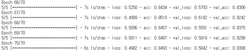
FCN-16
history_fcn16 = model_fcn16.fit(training_dataset,
                                steps_per_epoch=steps_per_epoch,
                                validation_data=validation_dataset,
                                validation_steps=validation_steps,
                                epochs=EPOCHS)
FCN-8
history_fcn8 = model_fcn8.fit(training_dataset,
                              steps_per_epoch=steps_per_epoch,
                              validation_data=validation_dataset,
                              validation_steps=validation_steps,
                              epochs=EPOCHS)
Evaluate the Model
validation dataset의 ground truth image와 label map를 우선 읽어옵니다.
def get_images_and_segments_test_arrays():
    '''
    Gets a subsample of the val set as your test set

    Returns:
        Test set contatining ground truth images and label maps
    '''

    y_true_segments = []
    y_true_images = []
    test_count = 64

    ds = validation_dataset.unbatch()
    ds = ds.batch(101)

    for image, annotation in ds.take(1):
        y_true_images = image
        y_true_segments = annotation

    y_true_segments = y_true_segments[:test_count, :, :, :]
    y_true_segments = np.argmax(y_true_segments, axis=3)

    return y_true_images, y_true_segments

# load the ground truth images and segmentation masks
y_true_images, y_true_segments = get_images_and_segments_test_arrays()
model의 prediction을 얻습니다. 결과는 softmax output으로 각 클래스의 확률이므로, 가장 높은 확률을 인덱스만을 취합니다.
# get the model prediction
results_fcn32 = model_fcn32.predict(validation_dataset, steps=validation_steps)
results_fcn16 = model_fcn16.predict(validation_dataset, steps=validation_steps)
results_fcn8 = model_fcn8.predict(validation_dataset, steps=validation_steps)

# for each pixel, get the slice number which has the highest probaility
results_fcn32 = np.argmax(results_fcn32, axis=3)
results_fcn16 = np.argmax(results_fcn16, axis=3)
results_fcn8 = np.argmax(results_fcn8, axis=3)
모델을 평가하기 위해 IoU와 Dice Score를 계산하는 함수를 정의하고 평가해보도록 하겠습니다.
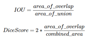
IoU(Intersection over Union)은 true label와 pred label의 겹치는 부분의 넓이를 두 라벨이 차지하는 넓이로 나누어준 값으로, 0~1 사이의 값을 갖습니다.
Dice Score는 라벨의 겹치는 부분의 넓이를 두 라벨의 각각의 넓이를 합한 값으로 나누어서 2를 곱한 값이며, 이값 또한 0~1 사이의 값을 갖습니다.
두 평가지표는 모두 이미지나 영상처리에서 사용되는 지표로 1에 가까울수록 segmentation이 잘 되었다는 것을 의미합니다.
def compute_metrics(y_true, y_pred):
    '''
    Compute IoU and Dice Score

    Args:
        y_true(tensor) -- ground truth label map
        y_pred(tensor) -- predicted label map
    '''

    class_wise_iou = []
    class_wise_dice_score = []

    smoothening_factor = 0.00001

    for i in range(12):
        intersection = np.sum((y_pred == i) * (y_true == i))
        y_true_area = np.sum((y_true == i))
        y_pred_area = np.sum((y_pred == i))
        combined_area = y_true_area + y_pred_area

        iou = (intersection + smoothening_factor) / (combined_area - intersection + smoothening_factor)
        class_wise_iou.append(iou)

        dice_score = 2*((intersection + smoothening_factor) / (combined_area + smoothening_factor))
        class_wise_dice_score.append(dice_score)

    return class_wise_iou, class_wise_dice_score
이제 결과의 IoU와 Dice Score를 구하고, 예측결과를 살펴보도록 하겠습니다.
# input a number from 0 to 63 to pick an image from the test set
integer_slider = 20
# compute metrics
iou_fcn32, dice_score_fcn32 = compute_metrics(y_true_segments[integer_slider], results_fcn32[integer_slider])
iou_fcn16, dice_score_fcn16 = compute_metrics(y_true_segments[integer_slider], results_fcn16[integer_slider])
iou_fcn8, dice_score_fcn8 = compute_metrics(y_true_segments[integer_slider], results_fcn8[integer_slider])
# visualize the output and metrics
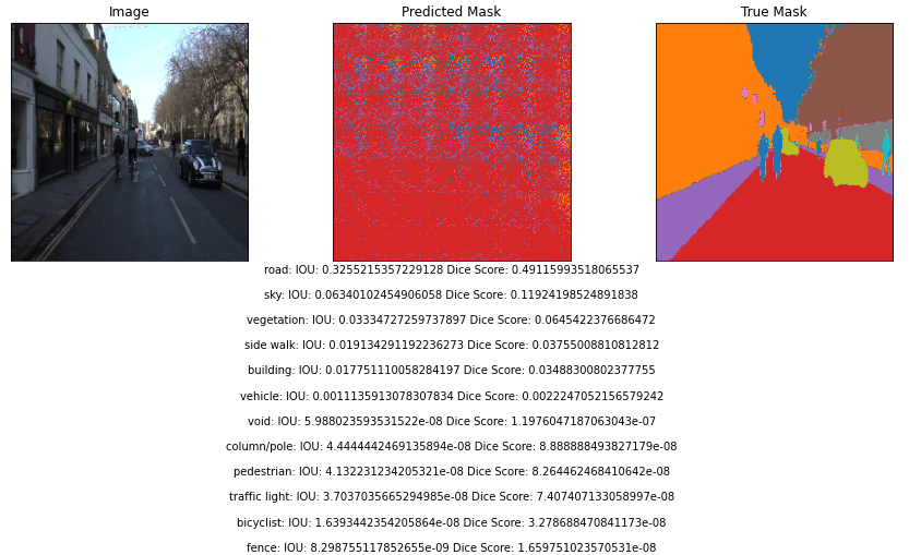
show_predictions(y_true_images[integer_slider], [results_fcn32[integer_slider], y_true_segments[integer_slider]], ["Image", "Predicted Mask", "True Mask"], iou_fcn32, dice_score_fcn32)
show_predictions(y_true_images[integer_slider], [results_fcn16[integer_slider], y_true_segments[integer_slider]], ["Image", "Predicted Mask", "True Mask"], iou_fcn16, dice_score_fcn16)
show_predictions(y_true_images[integer_slider], [results_fcn8[integer_slider], y_true_segments[integer_slider]], ["Image", "Predicted Mask", "True Mask"], iou_fcn8, dice_score_fcn8)
FCN-32
FCN-16

FCN-8

FCN-32와 FCN-16 모델은 학습이 크게 되지 않은 것으로 보이긴하지만, FCN-8보다 현저하게 해상도가 떨어지는 모습을 보여주고 있습니다. FCN-8의 경우에는 아주 정확하지는 않지만, 대체로 큼지막한 구역들은 정상적으로 구분하고 있습니다.
마지막으로 클래스 별로 각 모델들의 IoU와 Dice Score을 계산해보도록 하겠습니다.
# compute class-wise metrics
cls_wise_iou_fcn32, cls_wise_dice_score_fcn32 = compute_metrics(y_true_segments, results_fcn32)
cls_wise_iou_fcn16, cls_wise_dice_score_fcn16 = compute_metrics(y_true_segments, results_fcn16)
cls_wise_iou_fcn8, cls_wise_dice_score_fcn8 = compute_metrics(y_true_segments, results_fcn8)
IoU
# print IOU for each class
print('FCN-32')
for idx, iou in enumerate(cls_wise_iou_fcn32):
    spaces = ' ' * (13-len(class_names[idx]) + 2)
    print("{}{}{} ".format(class_names[idx], spaces, iou))
print('FCN-16')
for idx, iou in enumerate(cls_wise_iou_fcn16):
    spaces = ' ' * (13-len(class_names[idx]) + 2)
    print("{}{}{} ".format(class_names[idx], spaces, iou))
print('FCN-8')
for idx, iou in enumerate(cls_wise_iou_fcn8):
    spaces = ' ' * (13-len(class_names[idx]) + 2)
print("{}{}{} ".format(class_names[idx], spaces, iou)) 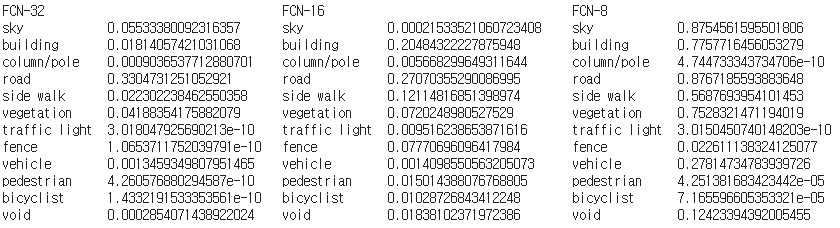
Dice Score
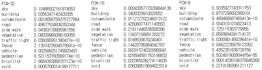
FCN-8이 확실히 높은 점수를 얻고 있습니다.
'ML & DL > tensorflow' 카테고리의 다른 글
| Class Activation Map(CAM) (6) | 2021.01.18 |
|---|---|
| [tensorflow] UNet (Oxford-IIIT Pet segmentation) (3) | 2021.01.17 |
| Breast Cancer Prediction (0) | 2021.01.13 |
| [tensorflow] GradientTape (0) | 2021.01.12 |
| [tensorflow] Custom Training Loops (tf.GradientTape) (1) | 2021.01.12 |


댓글