(tensorflow v2.4.0)
오래전부터 CNN Model을 해석하기 위한 방법을 찾아왔습니다.
이전에는 주로 filter들을 시각화하거나 filter가 최대로 활성화하는 입력을 찾는 등의 filter 단위의 해석이 많았고, 실제 모델이 이미지의 어떤 부분을 보고 예측하는지는 알 수 없었습니다.
하지만, Class Activation Map(CAM, paper)을 사용하면서 모델이 이미지의 어떤 부분을 보고 판단을 내리는지 어느 정도 알아낼 수 있습니다. 바로 아래처럼 말이죠.

Class Activation Map은 다음과 같이 구할 수 있습니다.
기본적인 Conv layer - Pooling layer의 구조를 쌓고 Feature들을 추출합니다. 그리고 CNN 구조 마지막에 Feature map을 펼쳐주는(Flatten) 것이 아닌, Global Average Pooling(GAP)를 사용합니다.
그리고 일반적인 구조와 동일하게 FC layer를 통해서 class를 예측(softmax output)하도록 합니다.
여기서 CAM은 마지막 conv layer와 FC layer의 weights를 사용해서 구하게 됩니다.
여기서 FC layer의 weight는 각 class에 대한 feature weight가 되며, 이 weights는 각 class의 feature vector들을 가지고 있는 것이죠.
그래서 마지막 Conv layer의 feature map과 FC layer의 weight를 곱해서 합해서 살펴보면, 모델이 이미지의 어떤 부분을 보고 class를 분류했는지 알 수 있게 됩니다.
위 내용을 tensorflow를 통해서 직접 살펴보도록 하겠습니다. pre-trained VGG16를 사용하고, cats vs dogs dataset을 사용했습니다.
Import
import tensorflow as tf import tensorflow_datasets as tfds import numpy as np import matplotlib.pyplot as plt import scipy as sp import cv2
Download and prepare the dataset
# Cats vs Dogs Dataset tfds.disable_progress_bar() splits = ['train[:80%]', 'train[80%:90%]', 'train[90%:]'] # load the dataset given the splits defined above splits, info = tfds.load('cats_vs_dogs', with_info=True, as_supervised=True, split = splits) (train_examples, validation_examples, test_examples) = splits num_examples = info.splits['train'].num_examples num_classes = info.features['label'].num_classes BATCH_SIZE = 32 def normalize_and_resize(image, label): image = tf.cast(image, tf.float32) image = image / 255. image = tf.image.resize(image, (224, 224)) return image, label # prepare batches train_batches = train_examples.shuffle(num_examples // 4).map(normalize_and_resize).batch(BATCH_SIZE).prefetch(tf.data.experimental.AUTOTUNE) validation_batches = validation_examples.map(normalize_and_resize).batch(BATCH_SIZE).prefetch(tf.data.experimental.AUTOTUNE) test_batches = test_examples.map(normalize_and_resize).batch(1)
train/valid/test dataset을 준비합니다.
Modeling and Train
def build_model(): base_model = tf.keras.applications.VGG16(input_shape= (224, 224, 3), weights='imagenet', include_top=False) # add a GAP layer output = tf.keras.layers.GlobalAveragePooling2D()(base_model.output) # output has two neurons for the 2 classes(dogs and cats) output = tf.keras.layers.Dense(2, activation='softmax')(output) # set the inputs and outputs of the model model = tf.keras.Model(base_model.input, output) for layer in base_model.layers[:-4]: layer.trainable = False model.compile(optimizer=tf.keras.optimizers.RMSprop(0.001), loss='sparse_categorical_crossentropy', metrics=['acc']) model.summary() return model model = build_model()
top의 classifier을 제외한 VGG16 모델을 불러오고, classifier는 GAP와 Dense layer로 구성합니다.
그리고, 10 Epochs 학습을 진행해줍니다. 5 Epochs로도 충분할 것 같습니다.
EPOCHS = 10 model.fit(train_batches, epochs=EPOCHS, validation_data=validation_batches)
Class Activation Map(CAM)
먼저 Dense layer의 weight와 마지막 Conv layer(block5_conv3)을 output으로 하는 cam_model을 정의하고, CAM을 이미지로 보여주는 함수를 정의하도록 하겠습니다.
cam_model = tf.keras.Model(model.input, outputs=(model.layers[-3].output, model.layers[-1].output)) cam_model.summary()
기본 model과 동일하지만, 마지막 conv layer인 block5_conv3의 feature map도 output으로 출력하는 것이 다릅니다.
사용될 GAP weight인 Dense layer의 weight를 간단하게 살펴보겠습니다. bias weight는 무시합니다.
gap_weights = model.layers[-1].get_weights()[0] gap_weights.shape

마지막 conv layer의 feature map의 모양이 (7, 7, 512) 이고 GAP를 통해 (512, )의 모양을 가지고, 최종 output은 2개의 class에 대한 확률이므로, Dense layer의 weights는 (512, 2)의 모양을 갖습니다. 여기서 1열은 class 0(cats)의 feature vector이며, 2열은 class 1(dogs)의 feature vector가 됩니다.
다음은 CAM을 나타내주는 함수입니다.
def show_cam(image_value, features, results, label): ''' Displays the class activation map of an image Args: image_value (tensor) -- preprocessed input image with size 224 x 224 features (array) -- features of the image, shape (1, 7, 7, 512) results (array) -- output of the sigmoid layer ''' features_for_img = features[0] prediction = results[0] class_activation_weigths = gap_weights[:,label] class_activation_features = sp.ndimage.zoom(features_for_img, (224/7, 224/7, 1), order=2) cam_output = np.dot(class_activation_features, class_activation_weigths) cam_output = tf.reshape(cam_output, (224,224)) # visualize the results print(f'sigmoid output: {results}') print(f"prediction: {'dog' if tf.argmax(results[0]) else 'cat'}") plt.figure(figsize=(8,8)) plt.imshow(cam_output, cmap='jet', alpha=0.5) plt.imshow(tf.squeeze(image_value), alpha=0.5) plt.show()
input image와 cam_model을 통한 결과 feature map과 prediction을 파라미터로 입력받고, 원래는 마지막 gap_weights와 feature map을 내적해주고 모두 더해줍니다(element-wise).
여기서는 예측하는 label의 weight vector만을 내적하겠습니다. 그래서 실제 이미지 위에 CAM을 나타내고, 해당 클래스를 높은 확률로 예측할 때 어디를 보는지 살펴보겠습니다.
# preprocess the test images augmented_test_data = test_examples.map(normalize_and_resize) test_batches = augmented_test_data.batch(1)
그럼 이제 test 이미지를 통해서 CAM이 무엇을 보여주는지 살펴보겠습니다.
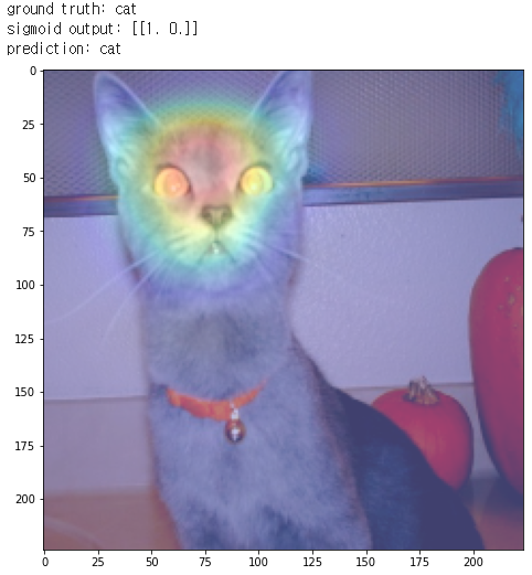
for img, lbl in test_batches.take(5): print(f"ground truth: {'dog' if lbl else 'cat'}") features,results = cam_model.predict(img) show_cam(img, features, results, lbl)
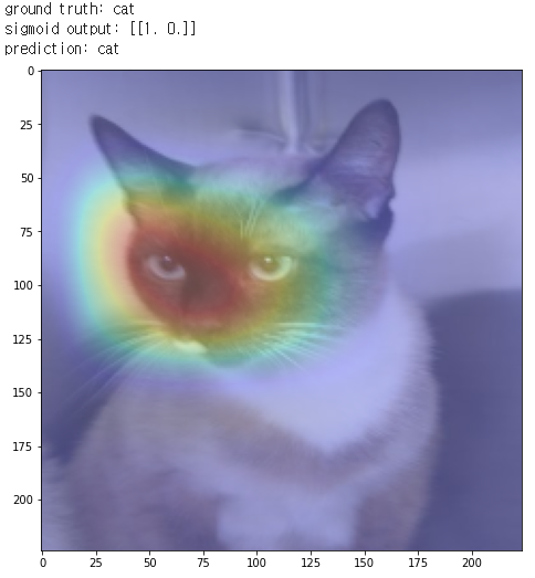
고양이의 얼굴을 중점적으로 보고 있다는 것을 의미합니다. 빨간색일수록 더 집중하고 있는 것이죠.
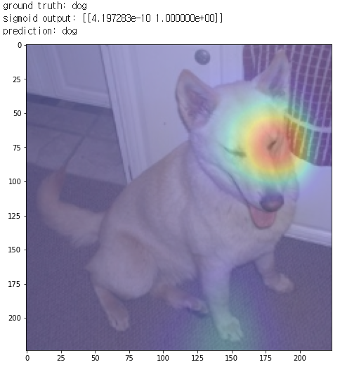
개 이미지도 동일합니다. feature map과 weights의 0열 vector가 곱해졌으며, 개의 얼굴을 주로 보고 있고, 앞발도 조금 보고 있는 것 같습니다.
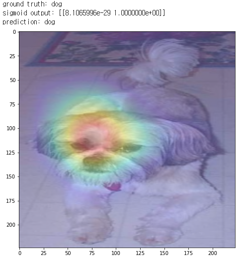
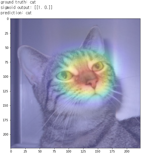
나머지 이미지들도 동일합니다.
'ML & DL > tensorflow' 카테고리의 다른 글
| Saliency Map (0) | 2021.01.18 |
|---|---|
| [tensorflow] UNet (Oxford-IIIT Pet segmentation) (3) | 2021.01.17 |
| [tensorflow] Fully Convolutional Networks(FCNs) (7) | 2021.01.16 |
| Breast Cancer Prediction (0) | 2021.01.13 |
| [tensorflow] GradientTape (0) | 2021.01.12 |


댓글