(tensorflow v2.4.0)
2021/01/12 - [ML & DL/tensorflow] - [tensorflow] Custom Training Loops (tf.GradientTape)
[tensorflow] Custom Training Loops (tf.GradientTape)
(tensorflow v2.4.0) 일반적으로 딥러닝 모델을 학습할 때, Build in Solution인 model.compile()과 model.fit()을 많이 사용합니다. model.compile()을 통해서 optimizer와 loss를 지정하고, model.fit()을 통해..
junstar92.tistory.com
이전 게시글에서 GradientTape를 사용해서 API가 아닌 직접 Training loop를 구현하여 모델의 학습을 진행했습니다.
이 방법으로 이번에는 Breast Cancer(유방암)을 예측하는 모델을 데이터 로드 및 전처리부터 학습 및 평가까지 순차적으로 진행해보겠습니다.
1. Import and Data load/preprocess
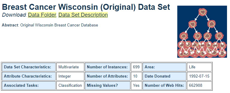
사용되는 Data는 UCI에서 제공하고 있으며, link를 참조하시기 바랍니다 !
import tensorflow as tf
import numpy as np
import matplotlib.pyplot as plt
import matplotlib.ticker as mticker
import pandas as pd

from sklearn.model_selection import train_test_split
from sklearn.metrics import confusion_matrix
import itertools

URL = "https://archive.ics.uci.edu/ml/machine-learning-databases/breast-cancer-wisconsin/breast-cancer-wisconsin.data"
data_file = tf.keras.utils.get_file("breast_cancer.csv", URL)
col_names = ["id", "clump_thickness", "un_cell_size", "un_cell_shape", "marginal_adheshion", "single_eph_cell_size", "bare_nuclei", "bland_chromatin", "normal_nucleoli", "mitoses", "class"]
df = pd.read_csv(data_file, names=col_names, header=None)
Download URL을 통해서 파일을 읽고, pandas를 통해 data를 읽어옵니다. Data는 아래 정보를 담고 있습니다.

df.head()
id는 사용하지 않기 때문에 id열은 삭제하고, 데이터의 간략한 정보를 살펴보겠습니다. 모든 data가 수치형으로 보이는데, 실제로 수치형인지 확인하기 위함입니다.
df.pop("id")
df.info()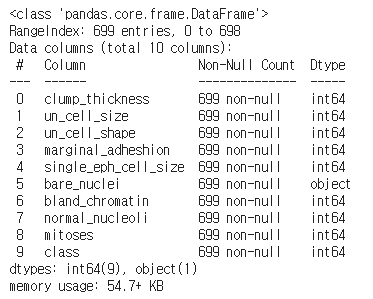
총 699개의 samples이 있으며, 데이터를 살펴보면 bare_nuclei의 data type이 object인 것을 확인할 수 있습니다. 수치가 아닌 다른 타입의 정보가 있다는 의미입니다. 실제로 살펴보면 '?'라는 정보가 있으며, 학습시에 이 정보는 어떻게 처리할 지 애매하므로, bare_nuclei의 값이 '?'인 샘플은 제거하도록 합니다.
df = df[df['bare_nuclei'] != '?']
df['bare_nuclei'] = pd.to_numeric(df['bare_nuclei'])
df.info()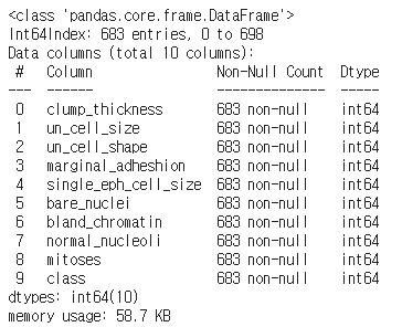
'?'를 가진 샘플을 제거하고, 수치형으로 타입을 바꿔준 결과입니다. 최종적으로 683개의 데이터가 사용됩니다.
다음으로 class 열을 살펴보도록 하겠습니다.
df['class'].hist(bins=20)
클래스의 값은 2와 4로 구분되어 있습니다. Binary Classification이므로, 0과 1로 label 값을 지정해주도록 하겠습니다.
참고로 2는 benign(양성)를 의미하고, 4는 malignant(악성)를 의미합니다.
# benign(2.0) => 0 // malignant(4.0) => 1
df['class'] = np.where(df['class'] == 2, 0, 1)
train/test data split and normalization
train/test set으로 dataset을 분리하고, normalization을 적용합니다. pandas의 describe 메소드를 통해서 각 열의 평균과 표준편차를 구해서 normalization을 적용합니다.
# split train/test set and get train stats
train, test = train_test_split(df, test_size=0.2)

train_stats = train.describe()
train_stats.pop('class')
train_stats = train_stats.transpose()

# get lables of train/test
train_Y = np.array(train.pop('class'), np.float64)
test_Y = np.array(test.pop('class'))

# normalization
norm_train_X = (train - train_stats['mean']) / train_stats['std']
norm_test_X = (test - train_stats['mean']) / train_stats['std']
norm_train_X = np.array(norm_train_X)
norm_test_X = np.array(norm_test_X)
Create tensorflow Dataset
tf.data.Dataset의 from_tensor_slices 메소드를 통해서 tensorflow dataset을 생성합니다. 그리고 train dataset에는 shuffle과 batch size를 적용하고, valid dataset에는 batch size만 적용해줍니다.
# create Tensorflow datatset
batch_size = 32

train_dataset = tf.data.Dataset.from_tensor_slices((norm_train_X, train_Y))
test_dataset = tf.data.Dataset.from_tensor_slices((norm_test_X, test_Y))

# shuffle and prepare batched dataset
train_dataset = train_dataset.shuffle(buffer_size=len(train)).batch(batch_size)
test_dataset = test_dataset.batch(batch_size)print(iter(train_dataset).__next__()) 를 통해서 어떻게 출력되는지 확인할 수 있습니다.
2. Define the model / optimizer / loss
모델을 정의하고 적용할 optimizer와 loss를 설정합니다.
def base_model():
    inputs = tf.keras.layers.Input(shape=(len(train.columns)))
    x = tf.keras.layers.Dense(128, activation='relu')(inputs)
    x = tf.keras.layers.Dense(64, activation='relu')(x)
    outputs = tf.keras.layers.Dense(1, activation='sigmoid')(x)
    model = tf.keras.Model(inputs, outputs)

    return model

model = base_model()
model.summary()
모델은 매우 간단한 구조이며, Dense layer로만 이루어진 네트워크입니다.
optimizer = tf.keras.optimizers.RMSprop(learning_rate=0.001)
loss_fn = tf.keras.losses.BinaryCrossentropy()
optimizer는 RMSprop(learning rate = 0.001), loss function으로는 Binary crossentropy 입니다.
학습을 진행하기 전에 학습되지 않은 모델의 결과를 confusion matrix를 통해서 확인해보겠습니다.
# plot confusion matrix to visualize the true outputs against the outputs predicted by the model
def plot_confusion_matrix(y_true, y_pred, title='', labels=[0,1]):
    cm = confusion_matrix(y_true, y_pred)
    fig = plt.figure()
    ax = fig.add_subplot(1,1,1)
    cax = ax.matshow(cm)
    plt.title(title)
    fig.colorbar(cax)
    ax.set_xticklabels([''] + labels)
    ax.set_yticklabels([''] + labels)
    plt.xlabel('Predicted')
    plt.ylabel('True')
    fmt = 'd'
    thresh = cm.max() / 2.
    for i, j in itertools.product(range(cm.shape[0]), range(cm.shape[1])):
          plt.text(j, i, format(cm[i, j], fmt),
                  horizontalalignment="center",
                  color="black" if cm[i, j] > thresh else "white")
    plt.show()

plot_confusion_matrix(test_Y, tf.round(outputs), title='Confusion Matrix for Untrained Model')
True 실제 label을 의미하고, Predicted는 모델이 예측한 label을 의미합니다. 학습이 제대로 이루어진다면, 1,3사분면의 개수는 줄어들고, 2,4사분면의 개수는 증가하게 될 것입니다.
3. Define Metrics (F1 score)
모델 평가를 위해서 F1 score를 사용할 예정이므로, tf.keras.metrics.Metric을 상속받아서 F1 score 클래스를 구현하였습니다. F1 score는 Precision과 Recall의 조화 평균으로 계산할 수 있습니다.
class F1Score(tf.keras.metrics.Metric):
    def __init__(self, name='f1_score', **kwargs):
        super(F1Score, self).__init__(name=name, **kwargs)

        # initialize required variables
        self.tp = tf.Variable(0, dtype=tf.int32) # true positive
        self.fp = tf.Variable(0, dtype=tf.int32) # false positive
        self.tn = tf.Variable(0, dtype=tf.int32) # true negative
        self.fn = tf.Variable(0, dtype=tf.int32) # false negative

    def update_state(self, y_true, y_pred, sample_weight=None):
        conf_matrix = tf.math.confusion_matrix(y_true, y_pred, num_classes=2)

        self.tn.assign_add(conf_matrix[0][0])
        self.tp.assign_add(conf_matrix[1][1])
        self.fp.assign_add(conf_matrix[0][1])
        self.fn.assign_add(conf_matrix[1][0])

    def result(self):
        # calculate precision
        if (self.tp + self.fp == 0):
            precision = 1.0
        else:
            precision = self.tp / (self.tp + self.fp)

        # calculate recall
        if (self.tp + self.fn == 0):
            recall = 1.0
        else:
            recall = self.tp / (self.tp + self.fn)

        f1_score = 2*(precision*recall) / (precision+recall)

        return f1_score

    def reset_states(self):
        self.tp.assign(0)
        self.tn.assign(0)
        self.fp.assign(0)
        self.fn.assign(0)
Metric 클래스를 상속받고, update_state, result, reset_states 함수를 오버라이딩하여 새롭게 정의합니다. __init__ 함수에서는 F1 score에서 필요한 값들을 저장할 수 있는 변수를 생성합니다.
오버라이딩 함수들에 대해서 간단하게 설명하면, update_state에서는 tf.math.confusion_matrix 메소드를 통해서 True Positive/True Negative/False Positive/False Negative 값을 얻고, 클래스 변수에 업데이트해줍니다.
그리고 result에서 수집한 결과값들을 통해 F1 score를 계산합니다.
마지막으로 reset_states는 Metric 결과를 초기화해줍니다.
train과 valid에서 사용되는 F1 score metric 객체와 정확도를 측정하기 위한 객체를 각각 생성해줍니다.
train_f1score_metric = F1Score()
valid_f1score_metric = F1Score()

train_acc_metric = tf.keras.metrics.BinaryAccuracy()
valid_acc_metric = tf.keras.metrics.BinaryAccuracy()
4. Train loop 구현
먼저 gradient를 계산하고, 적용하는 함수를 구현합니다.
def apply_gradient(model, optimizer, loss_fn, x, y):
    with tf.GradientTape() as tape:
        logits = model(x)
        loss = loss_fn(y, logits)

    gradients = tape.gradient(loss, model.trainable_weights)
    optimizer.apply_gradients(zip(gradients, model.trainable_weights))

    return logits, loss
다음은 한 epoch에서 진행되는 step loop를 위한 함수 구현입니다.
def train_for_one_epoch(train_dataset, model, optimizer, loss_fn, train_acc_metric, train_f1socre_metric, verbose=True):
    losses = []

    for step, (x_batch, y_batch) in enumerate(train_dataset):
        logits, loss = apply_gradient(model, optimizer, loss_fn, x_batch, y_batch)
        losses.append(loss)

        logits = tf.round(logits)
        logits = tf.cast(logits, tf.int64)

        train_acc_metric.update_state(y_batch, logits)
        train_f1score_metric.update_state(y_batch, logits)

        if verbose:
            print(f"Training loss for step {step}: {loss:.4f}")

    return losses
마지막으로 validation 수행을 위한 loop 함수입니다.
def perform_validation(test_dataset, model, loss_fn, valid_acc_metric, valid_f1score_metric):
    losses = []

    for x_batch, y_batch in test_dataset:
        val_logits = model(x_batch)
        val_loss = loss_fn(y_batch, val_logits)
        losses.append(val_loss)

        val_logits = tf.cast(tf.round(val_logits), tf.int64)

        valid_acc_metric.update_state(y_batch, val_logits)
        valid_f1score_metric.update_state(y_batch, val_logits)

    return losses
5. Training
학습을 진행해보도록 하겠습니다. 5 epoch 동안 학습을 진행하였습니다.
epochs = 5
epochs_val_losses, epochs_train_losses = [], []

for epoch in range(epochs):
    print(f'Start of epoch {epoch+1},')

    # train
    losses_train = train_for_one_epoch(train_dataset, model, optimizer, loss_fn, train_acc_metric, train_f1score_metric)

    # Get result from training metrics
    train_acc = train_acc_metric.result()
    train_f1score = train_f1score_metric.result()

    # Perform validation
    losses_val = perform_validation(test_dataset, model, loss_fn, valid_acc_metric, valid_f1score_metric)

    # Get result from validation metrics
    valid_acc = valid_acc_metric.result()
    valid_f1score = valid_f1score_metric.result()

    #Calculate training and validation losses for current epoch
    losses_train_mean = np.mean(losses_train)
    losses_valid_mean = np.mean(losses_val)
    epochs_val_losses.append(losses_valid_mean)
    epochs_train_losses.append(losses_train_mean)

    print(f'\n Epoch {epoch+1}: \nTrain loss: {losses_train_mean:.4f}, Train Accuracy: {train_acc:.4f}, Train F1 Score: {train_f1score:.4f}\nValid loss: {losses_valid_mean:.4f}, Valid Accuracy: {valid_f1score:.4f}, Valid F1 Score: {valid_f1score:.4f}')

    # reset metrics
    train_acc_metric.reset_states()
    train_f1score_metric.reset_states()
    valid_acc_metric.reset_states()
    valid_f1score_metric.reset_states()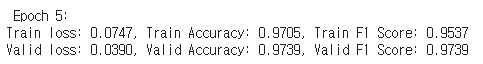
train과 valid dataset에서 모두 약 97%의 정확도와 0.95~0.97의 F1 Score를 얻었습니다.
6. Evaluate the model
def plot_metrics(train_metric, valid_metric, metric_name, title, ylim=5):
    plt.title(title)
    plt.ylim(0, ylim)
    plt.gca().xaxis.set_major_locator(mticker.MultipleLocator(1))
    plt.plot(train_metric, color='blue', label=metric_name)
    plt.plot(valid_metric, color='green', label='val_' + metric_name)
    plt.legend()

plot_metrics(epochs_train_losses, epochs_val_losses, "Loss", "Loss", ylim=0.5)
학습동안의 loss의 변화입니다. loss가 수렴하고 있는 것을 확인할 수 있습니다.
마지막으로 confusion matrix를 통해서 결과를 확인해보도록 하겠습니다.
test_outputs = model(norm_test_X)
plot_confusion_matrix(test_Y, tf.round(test_outputs), title='Confusion Matrix for Untrained Model')
총 137개의 샘플 중에서 3개만 잘못 예측하고, 나머지는 올바르게 예측한 것을 확인할 수 있습니다.
- 참조
Coursera - Custom and Distributed Training with Tensorflow : Week 2
'ML & DL > tensorflow' 카테고리의 다른 글
| [tensorflow] UNet (Oxford-IIIT Pet segmentation) (3) | 2021.01.17 |
|---|---|
| [tensorflow] Fully Convolutional Networks(FCNs) (7) | 2021.01.16 |
| [tensorflow] GradientTape (0) | 2021.01.12 |
| [tensorflow] Custom Training Loops (tf.GradientTape) (1) | 2021.01.12 |
| [tensorflow] Custom Model (Mini ResNet, VGGNet 구현) (1) | 2021.01.12 |


댓글