해당 내용은 Coursera의 딥러닝 특화과정(Deep Learning Specialization)의 다섯 번째 강의 Recurrent Neural Network를 듣고 정리한 내용입니다. (Week 3)

3주차 실습 중의 하나는 Attention 모델이 포함된 Neural Machine Translation(NMT) 구현입니다.
이번 실습에서는 human-readable dates를 machine-readable dates로 변환하는 모델을 구현할 예정입니다.
human-readable dates는 '25th of June, 2009'와 같이 영어와 숫자 등이 섞여 있는 형태이며, machine-readable dates는 '2009-06-25'와 같이 숫자와 '-' 대쉬가 섞여있는 형태입니다.
사용되는 package
import numpy as np import random from faker import Faker # 가짜 데이터 생성을 위한 package from tqdm import tqdm # 상태bar 표시 package from babel.dates import format_date # 날짜 포맷 설정을 위한 package import tensorflow as tf
1. Dataset
모델 구현에 앞서, 10000개의 human-readable dates와 machine-readable dates를 생성합니다. 두 dates는 서로 같은 날짜를 나타냅니다.
우선 난수 설정을 해주고, 사용할 format을 정의합니다. 그리고, date를 읽는 load 함수를 정의합니다.
fake = Faker() Faker.seed(12345) random.seed(12345) # Define format of the data we would like to generate FORMATS = ['short', 'medium', 'long', 'full', 'full', 'full', 'full', 'full', 'full', 'full', 'full', 'full', 'full', 'd MMM YYY', 'd MMMM YYY', 'dd MMM YYY', 'd MMM, YYY', 'd MMMM, YYY', 'dd, MMM YYY', 'd MM YY', 'd MMMM YYY', 'MMMM d YYY', 'MMMM d, YYY', 'dd.MM.YY'] def load_date(): dt = fake.date_object() try: human_readable = format_date(dt, format=random.choice(FORMATS), locale='en_US') human_readable = human_readable.lower() human_readable = human_readable.replace(',', '') machine_readable = dt.isoformat() except AttributeError as e: return None, None, None return human_readable, machine_readable, dt def load_dataset(m): human_vocab = set() machine_vocab = set() dataset = [] Tx = 30 for i in tqdm(range(m)): h, m, _ = load_date() if h is not None: dataset.append((h, m)) human_vocab.update(tuple(h)) machine_vocab.update(tuple(m)) human = dict(zip(sorted(human_vocab) + ['<unk>', '<pad>'], list(range(len(human_vocab) + 2)))) inv_machine = dict(enumerate(sorted(machine_vocab))) machine = {v:k for k,v in inv_machine.items()} return dataset, human, machine, inv_machine
위 함수로 dataset을 생성해보도록 하겠습니다.
m = 10000 dataset, human_vocab, machine_vocab, inv_machine_vocab = load_dataset(m)
human_vocab는 human-readable date에서 사용되는 문자를 index로 변환해주는 딕셔너리이고, machine_vocab은 machine-readable date에 사용되는 문자를 index로 변환해주는 딕셔너리입니다. inv_machine_vocab은 machine-readable date의 인덱스를 문자로 변환해주는 딕셔너리입니다.
10개의 sample을 확인해봅시다.
print(len(dataset)) dataset[:10]
그리고, 모델의 입력으로 문자가 아닌 문자를 인덱스로 변환한 데이터를 사용할 것이기 때문에, 문자를 인덱스로 변환해주는 함수와 인덱스를 문자로 변환해주는 함수를 정의합니다. 문자를 인덱스로 변환하는 과정에서 대문자는 모두 소문자로 변환하고, 콤마(',')는 제거됩니다.
def string_to_int(string, length, vocab): """ Converts all strings in the vocabulary into a list of integers representing the positions of the input string's characters in the "vocab" Arguments: string -- input string, e.g. 'Wed 10 Jul 2007' length -- the number of time steps you'd like, determines if the output will be padded or cut vocab -- vocabulary, dictionary used to index every character of your "string" Returns: rep -- list of integers (or '<unk>') (size = length) representing the position of the string's character in the vocabulary """ string = string.lower() string = string.replace(',', '') if len(string) > length: string = string[:length] rep = list(map(lambda x: vocab.get(x, '<unk>'), string)) if len(string) < length: rep += [vocab['<pad>']] * (length - len(string)) #print (rep) return rep def int_to_string(ints, inv_vocab): """ Output a machine readable list of characters based on a list of indexes in the machine's vocabulary Arguments: ints -- list of integers representing indexes in the machine's vocabulary inv_vocab -- dictionary mapping machine readable indexes to machine readable characters Returns: l -- list of characters corresponding to the indexes of ints thanks to the inv_vocab mapping """ l = [inv_vocab[i] for i in ints] #print(l) return l
임의의 날짜로 테스트한 결과입니다.
print(string_to_int('sunday may 22 1988', len('sunday may 22 1988'), human_vocab)) print(int_to_string([2, 10, 9, 9, 0, 1, 6, 0, 3, 3], inv_machine_vocab))

그리고 전체 dataset을 전처리해주는 함수를 정의합니다.
def preprocess_data(dataset, human_vocab, machin_vocab, Tx, Ty): X, Y = zip(*dataset) X = np.array([string_to_int(i, Tx, human_vocab) for i in X]) Y = [string_to_int(t, Ty, machine_vocab) for t in Y] Xoh = np.array(list(map(lambda x: tf.keras.utils.to_categorical(x, num_classes=len(human_vocab)), X))) Yoh = np.array(list(map(lambda x: tf.keras.utils.to_categorical(x, num_classes=len(machine_vocab)), Y))) return X, np.array(Y), Xoh, Yoh
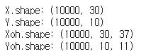
human-readable date는 길이 는 30으로 설정하고, output인 machine-readable date는 'YYYY-MM-DD'의 포맷이기 때문에 는 10으로 설정해서, 전체 dataset을 전처리해줍니다.
인덱스로 변환된 데이터는 keras.utils.to_categorical을 통해서 one hot 인코딩까지 진행해주어 반환합니다.
Tx = 30 # maximum length of the human readable date Ty = 10 # YYYY-MM-DD is 10 characters long. X, Y, Xoh, Yoh = preprocess_data(dataset, human_vocab, machine_vocab, Tx, Ty) print("X.shape:", X.shape) print("Y.shape:", Y.shape) print("Xoh.shape:", Xoh.shape) print("Yoh.shape:", Yoh.shape)
index 0의 데이터를 샘플로 확인해보도록 하겠습니다.
index = 0 print("Source date:", dataset[index][0]) print("Target date:", dataset[index][1]) print() print("Source after preprocessing (indices):", X[index]) print("Target after preprocessing (indices):", Y[index]) print() print("Source after preprocessing (one-hot):", Xoh[index]) print("Target after preprocessing (one-hot):", Yoh[index])
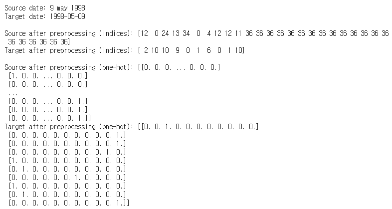
최대 길이보다 짧은 부분은 <pad>로 채워진 것을 볼 수 있습니다.
2. Model 구현
전체 모델 구성은 아래와 같습니다.
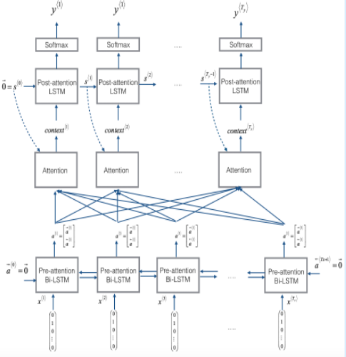
Bi-LSTM layer(Pre-attention) -> Attention -> LSTM layer(Post-attention) -> softmax -> output 의 순으로 모델이 수행됩니다.
2.1 Attention Mechanism
우선 Attention을 구현해보도록 합시다. 전체 모델을 보시면 Attention을 통해서 가 출력되고, 이 값은 다시 LSTM layer의 입력으로 사용되는 것을 볼 수 있습니다.
여기서 는 아래와 같이 계산됩니다.
위 과정이 tensorflow에서 어떻게 구현되는지 살펴보도록 합시다.
우선 attention 구현에 사용되는 layer들입니다.
# Defined shared layers as global variables repeator = tf.keras.layers.RepeatVector(Tx) concatenator = tf.keras.layers.Concatenate(axis=-1) densor1 = tf.keras.layers.Dense(10, activation = "tanh") densor2 = tf.keras.layers.Dense(1, activation = "relu") activator = tf.keras.layers.Activation('softmax', name='attention_weights') dotor = tf.keras.layers.Dot(axes = 1)
진행되는 과정은 다음과 같습니다.
Pre-attention Bi-LSTM의 hidden units을 , Post-attention의 LSTM의 hidden units을 라고 하겠습니다.
(Bi-LSTM의 activation 차원은 이며, 를 만족합니다.)
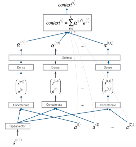
1. tf.keras.layers.RepeatVector를 통해 의 차원을 확장
Attention의 입력으로는 와 가 사용되는데, 과 각각의 과 concat해주기 위해서 우선 차원을 통일시켜줍니다. 각 에는 모두 동일한 가 합쳐지므로, concat하기 전에 의 차원을 에서 으로 확장해줍니다.
( 차원의 벡터가 Tx만큼 반복된것과 같습니다.)
2. tf.keras.layers.Concatenate를 통해서 과 를 합쳐줌
의 과 의 Bi-LSTM의 activation을 concat해주며, 그 결과는 차원의 벡터가 생성됩니다.
3. 합쳐준 concat을 Dense layer(1, 2)를 통해서 를 계산
2번 과정에서 concat 결과물을 Dense layer를 통해서 attention parameter 를 계산하기 전의 값 를 계산해줍니다. 두 개의 Dense 층을 통해서 결과적으로 의 벡터가 됩니다.
4. softmax layer를 통해서 attention parameter 를 계산
3번 과정에서의 결과 을 softmax layer를 통해서 attention parameter 을 계산합니다.
5. tf.keras.layers.Dot layer를 통해서 를 계산
이전 과정에서 계산된 과 pre-attention Bi-LSTM의 output인 를 사용해 을 계산합니다. 는 의 차원을 가지고, 은 의 차원을 가지므로, 계산 결과는 의 차원을 갖습니다.
위 과정이 아래 one_step_attention 함수에서 수행됩니다.
def one_step_attention(a, s_prev): """ Performs one step of attention: Outputs a context vector computed as a dot product of the attention weights "alphas" and the hidden states "a" of the Bi-LSTM. Arguments: a -- hidden state output of the Bi-LSTM, numpy-array of shape (m, Tx, 2*n_a) s_prev -- previous hidden state of the (post-attention) LSTM, numpy-array of shape (m, n_s) Returns: context -- context vector, input of the next (post-attention) LSTM cell """ ### START CODE HERE ### # Use repeator to repeat s_prev to be of shape (m, Tx, n_s) so that you can concatenate it with all hidden states "a" (≈ 1 line) s_prev = repeator(s_prev) # Use concatenator to concatenate a and s_prev on the last axis (≈ 1 line) # For grading purposes, please list 'a' first and 's_prev' second, in this order. concat = concatenator([a, s_prev]) # Use densor1 to propagate concat through a small fully-connected neural network to compute the "intermediate energies" variable e. (≈1 lines) e = densor1(concat) # Use densor2 to propagate e through a small fully-connected neural network to compute the "energies" variable energies. (≈1 lines) energies = densor2(e) # Use "activator" on "energies" to compute the attention weights "alphas" (≈ 1 line) alphas = activator(energies) # Use dotor together with "alphas" and "a" to compute the context vector to be given to the next (post-attention) LSTM-cell (≈ 1 line) context = dotor([alphas, a]) ### END CODE HERE ### return context
2.2 전체 Model 구현
그럼 이제 post-attention의 LSTM layer와 output layer를 정의하고, 전체 모델을 구성해보도록 하겠습니다.
로 설정했습니다.
n_a = 32 # number of units for the pre-attention, bi-directional LSTM's hidden state 'a' n_s = 64 # number of units for the post-attention LSTM's hidden state "s" # Please note, this is the post attention LSTM cell. post_activation_LSTM_cell = LSTM(n_s, return_state = True) # post-attention LSTM output_layer = Dense(len(machine_vocab), activation=softmax)
def model(Tx, Ty, n_a, n_s, human_vocab_size, machine_vocab_size): """ Arguments: Tx -- length of the input sequence Ty -- length of the output sequence n_a -- hidden state size of the Bi-LSTM n_s -- hidden state size of the post-attention LSTM human_vocab_size -- size of the python dictionary "human_vocab" machine_vocab_size -- size of the python dictionary "machine_vocab" Returns: model -- Keras model instance """ # Define the inputs of your model with a shape (Tx,) # Define s0 (initial hidden state) and c0 (initial cell state) # for the decoder LSTM with shape (n_s,) X = Input(shape=(Tx, human_vocab_size)) s0 = Input(shape=(n_s,), name='s0') c0 = Input(shape=(n_s,), name='c0') s = s0 c = c0 # Initialize empty list of outputs outputs = [] ### START CODE HERE ### # Step 1: Define your pre-attention Bi-LSTM. (≈ 1 line) a = Bidirectional(LSTM(n_a, return_sequences=True), input_shape=(m, Tx, n_a*2))(X) # Step 2: Iterate for Ty steps for t in range(Ty): # Step 2.A: Perform one step of the attention mechanism to get back the context vector at step t (≈ 1 line) context = one_step_attention(a, s) # Step 2.B: Apply the post-attention LSTM cell to the "context" vector. # Don't forget to pass: initial_state = [hidden state, cell state] (≈ 1 line) s, _, c = post_activation_LSTM_cell(context, initial_state=[s,c]) # Step 2.C: Apply Dense layer to the hidden state output of the post-attention LSTM (≈ 1 line) out = output_layer(s) # Step 2.D: Append "out" to the "outputs" list (≈ 1 line) outputs.append(out) # Step 3: Create model instance taking three inputs and returning the list of outputs. (≈ 1 line) model = Model(inputs=[X, s0, c0], outputs=outputs) ### END CODE HERE ### return model model = model(Tx, Ty, n_a, n_s, len(human_vocab), len(machine_vocab)) model.summary()
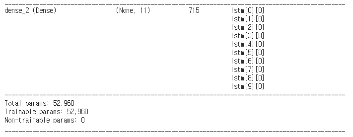
총 52,960의 파라미터를 갖는 모델입니다.
3. Model Compile & Learning
Adam Optimizer(learning rate = 0.005, , decay = 0.01)을 사용하고, metric는 'accuracy'로 모델을 컴파일해서 100 epoch 동안 학습을 진행해보겠습니다.
opt = tf.keras.optimizers.Adam(lr=0.005, beta_1=0.9, beta_2=0.999, decay=0.01) model.compile(optimizer=opt, loss='categorical_crossentropy', metrics=['accuracy']) s0 = np.zeros((m, n_s)) c0 = np.zeros((m, n_s)) outputs = list(Yoh.swapaxes(0,1)) model.fit([Xoh, s0, c0], outputs, epochs=100, batch_size=100)

최종 accuracy는 약 98.7%로 측정됩니다.
4. Test new samples
학습이 잘 이루어졌는데, 실제 새로운 데이터를 사용해서 테스트해보도록 하겠습니다.
학습에 사용하던 초기 activation과 candidate값은 training data 갯수에 해당하는 행렬이므로, s0과 c0을 그대로 사용하면 에러가 발생합니다. 1개의 batch size를 가진 zero-행렬로 변환한 후에 진행하면 에러없이 결과를 확인할 수 있습니다.
s0 = np.zeros((1, n_s)) c0 = np.zeros((1, n_s)) EXAMPLES = ['3 May 1979', '5 April 09', '21th of August 2016', 'Tue 10 Jul 2007', 'Saturday May 9 2018', 'March 3 2001', 'March 3rd 2001', '1 March 2001'] for example in EXAMPLES: source = string_to_int(example, Tx, human_vocab) source = np.array(list(map(lambda x: tf.keras.utils.to_categorical(x, num_classes=len(human_vocab)), source))) source = source[tf.newaxis,:,:] prediction = model.predict([source, s0, c0]) prediction = np.argmax(prediction, axis = -1) output = [inv_machine_vocab[int(i)] for i in prediction] print("source:", example) print("output:", ''.join(output),"\n")
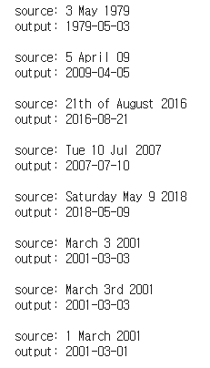
정상적으로 예측이 된 것을 볼 수 있습니다.
'Coursera 강의 > Deep Learning' 카테고리의 다른 글
| [Coursera] Deep Learning Specialization 강의 요약 (0) | 2020.12.31 |
|---|---|
| Sequence models & Attention mechnism / Speech recognition(CTC) (0) | 2020.12.28 |
| [실습] Operations on word vectors - Debiasing (0) | 2020.12.26 |
| NLP and Word Embeddings: Word2vec & GloVe (0) | 2020.12.26 |
| Introduction to Word Embeddings (0) | 2020.12.24 |


댓글